NEATO Gauntlet

The objective of this project (the final of my Olin class Quantitative Engineering Analysis) was to navigate a simulated Roomba-like robot through a world called The Gauntlet, avoiding obstacles (boxes) until finally reaching the goal (cylinder).
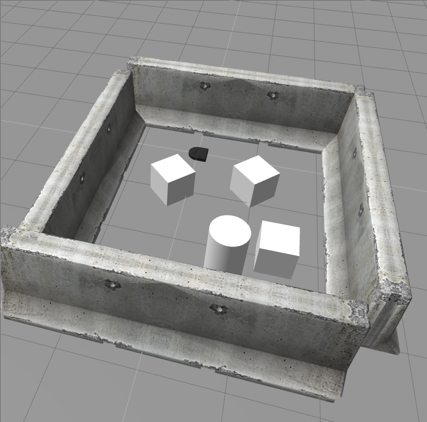
The Gauntlet
The Code
RANSAC
The RANSAC, or Random Sample Consensus algorithm is a method of identifying features from a dataset. It works by selecting a set of points and fitting a model to them. The algorithm then separates the original dataset into a set of inliers, which are points that fall within a threshold d of the model, and a set of outliers. The process is repeated n times until the algorithm has determined the best fit of the model, and outputs that.
At this point, RANSAC has output a single feature with a given set of inliers, and so it runs again with the leftover outliers to identify a second set of features, and then a third, and so on, until it has identified all the major features of the data.
Fitting Lines
To fit a line, the algorithm chooses two points:
| |
It calculates the vector between these two points and its orthogonal vector, and then for every other point in the dataset, it performs the dot product of the point and the unit orthogonal vector to get the perpendicular distance from the point to the line formed by P1 and P2:
| |
It also finds the biggest gap in the our model, because if it is too big, it should be discarded:
| |
Fitting Circles
Fitting circles is more challenging. When fitting lines, it is easy to just find the perpendicular distance from any point to that line, but with circles, I needed to be more clever.
A circle can be defined by three points, so the algorithm chooses 3 points from the dataset and splits them in x and y components:
| |
It then runs a linear regression in the form of a linear systems of equations to solve for the coefficients of the circle in general form:
| |
Once it has the center and radius of the circle, it calculates the distance from any point to the circle by finding the distance to the center of the circle, and subtracts the radius to get the distance from the edge of the circle:
| |
There are two issues that initially came up with this implementation:
- The algorithm would sometimes treat straight lines as arcs of circles with huge radii, on the scale of 106, and
- The circle would identify right angles as arcs of a circle.
To solve the first issue, since I knew the approximate size of the circle, I ruled out models with radii too far from the goal. That part was easier. The second issue required some more ingenuity.
In theory, if a set of data points fit a model, then any subset of those points would fit the same model just as well. I used this fact to solve the right-angle fitting issue by performing the RANSAC circle detection once more on the set of inliers generated the first time. If the original fit of a circle was correct, then the center and radius of the new circle will be roughly the same. However, if it is a right angle, it is more likely that the center of the newly generated circle will be significantly different from the original, so we can rule it out as a circle.
Generating Vector Fields
Now that I had a set of boundaries and a goal from our dataset, I needed a way to generate a map that the NEATO can follow. For this challenge, I implemented a vector field/gradient descent algorithm to have the NEATO navigate the gauntlet. To generate the map, I used the equation:
\[z = ln \sqrt{(x-x_n)^{2}+(y-y_n)^{2}}\]I added multiple of these terms together to generate a composite map of the NEATO’s surroundings. If the term is positive, then we get a “sink”, and if the term is negative we get a “source”. When it comes time for the NEATO to choose a path with gradient descent, it will be attracted to the sinks and repelled from the sources.
I took three different approaches to generating the sinks and sources. First, I just use the endpoints of the best fit lines as sources and the center of the circle as sinks. The issue with this was that on big lines, the NEATO would find paths through the middle of a wall, and would then collide with said wall.
The next thing I tried was having n points between the two endpoints of every line and making each of those sources. The problem there was in the density of sources. Longer lines, like the boundary of the Gauntlet, would have points spaced out every .25 meters, but short lines like the edge of a box would have points spaced out every .025 meters. This was an issue because boundaries need to all have the same weights or else the ones with less weight/density will be treated as acceptable for finding paths.
The final, successful, approach I took was instead calculating the length of the lines and generating a set of equally spaced points along the line to create sources. For the circle, I found equally spaced points around the circumference.
The final equation was:
…complicated. I like to embed mathematics with \({\KaTeX}\)
, as you will see above. I knew the equation had a lot of sources and sinks (around 20,000), so instead of manually writing it all out, I wrote a Python script to automate it for me. In mathtex.py I import all the sources and sinks from CSV files and process them into LaTeX. My thinking was that I would then copy the result into Overleaf, a LaTeX compiler, but when I tried pasting into Overleaf, it said there was an error, and then my browser crashed. If you’d like to view the raw LaTeX, you can run python3 mathtex.py or you can look at the CSV files to see the points for yourself.
Gradient Descent
After I generated the equation, it was time to get the NEATO to actually move. In order to do this, I used a gradient descent method. The algorithm works by assessing the current position of the NEATO using ROS’s /odom topic (which gets the position of the NEATO and it’s orientation in the form of a quaternion), rotating in the opposite direction of the gradient vector at its current point, and then moving along some proportion of the length of the gradient vector.
The equation to calculate the next point is:
\[r_{n+1} = r_{n} - \lambda_{n} \cdot \nabla V\]where \( \lambda_{n} \) is a scalar and determined by \(\lambda_{n-1} = \delta \lambda_{n}\) and \(\delta\) is some scalar. The code to make the NEATO rotate is as follows:
| |
The code for making the NEATO travel in a straight line is very similar, except the wheels rotate in the same direction:
| |
In the end, the NEATO took approximately 45 seconds to reach its goal. It’s slowness is due in part to the slow wheel velocity of 0.2 m/s, and in part because it was doing so much computational work in between each movement.